[TL;DR] Energy-Based Transferability Estimation

Code Visualization Codde

@misc{gholami2023etranenergybasedtransferabilityestimation,
      title={ETran: Energy-Based Transferability Estimation}, 
      author={Mohsen Gholami and Mohammad Akbari and Xinglu Wang and Behnam Kamranian and Yong Zhang},
      year={2023},
      eprint={2308.02027},
      archivePrefix={arXiv},
      primaryClass={cs.CV},
      url={https://arxiv.org/abs/2308.02027}, 
}

What (is it)?

ETran was proposed on the hypothesis that evaluating whether target dataset features are in-distribution (IND) or out-of-distribution (OOD) for a given PTM would be enough for a good Transferrability Estimation (TE) metric. The core idea works based off the concept of statistical physics that correlates energy of a system to the likelihood of a sample being present in the distribution the source model (\(\phi\)) is trained on.

Cool Stuff:

• Makes explainable estimations about the knowledge relationship between source model and target dataset;
• Outlines a way to deal with object detection tasks using bounding boxes;

The main part of the metric involves the idea behind Energy-Based Models (EBMs). EBMs are a class of models that use an energy function (may (or may not) be parameterized) to assign a scalar energy value to each possible configuration of the input data. It’s simple – anything that relates a low return value with good direction during training can be an energy function. For simpler models, this can be MSE or Cross-Entropy. If you’re getting more complex, certain layers or modules themselves should be made for this purpose.

At all levels, the energy function is used to derive a probability distribution through the Gibbs distribution. The below equation shows that the probability of a particular outcome \(y\) given the input \(x\) decreases exponentially with increasing energy \(E(x,y)\). Just replace \(E(x,y)\) here with your energy function above and you’re set to run some visualizations on your PTM (\(\phi\)).

Why (do we need it)?

• Previous methods (think pre-2023 including SDFA and NLEEP) typically fail when the target dataset diverges significantly from the source dataset’s distribution. When the target dataset is OOD compared to the pre-trained model, the extracted features can become unreliable. (Note the word unreliable – it means “not robust”, but can be right sometimes.)
• The effectiveness of these methods is often compromised by the differences in features before and after fine-tuning, due to variations in source and target domains.
• ETran is also more efficient (think 2x and more) because it does not require extensive label information or complex optimization processes. The energy score is label- and optimization-free, making it a fast and easy-to-use metric for transferability estimation.

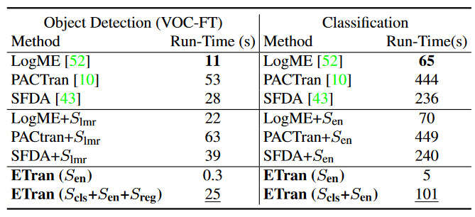
(Please read the When (does it fail)? section)

How (does it work)?

ETran’s transferability assessment includes three primary scores:

• Energy Score: Measures the likelihood of the target dataset being compatible with the pre-trained model.
• Classification Score: Uses LDA to project features into a higher D space, maximizing inter-class variance and minimizing intra-class variance.
• Regression Score: Uses SVD to evaluate the transferability for object detection tasks. Pretty interesting.

Energy Score \(S_{en}\):

The energy function here is the model’s embedding layer itself. Thus, the outputted features act as the energy scores. The final score is the mean of all energy scores for the samples.

Here is an optimized view of the process:

where,

• \(f_{ij}\): feature_vector[i][j] (\(i\) is the sample number and \(j\) is the vector dimension),
• \(d\): n_dim,
• \(C\): n_samples,

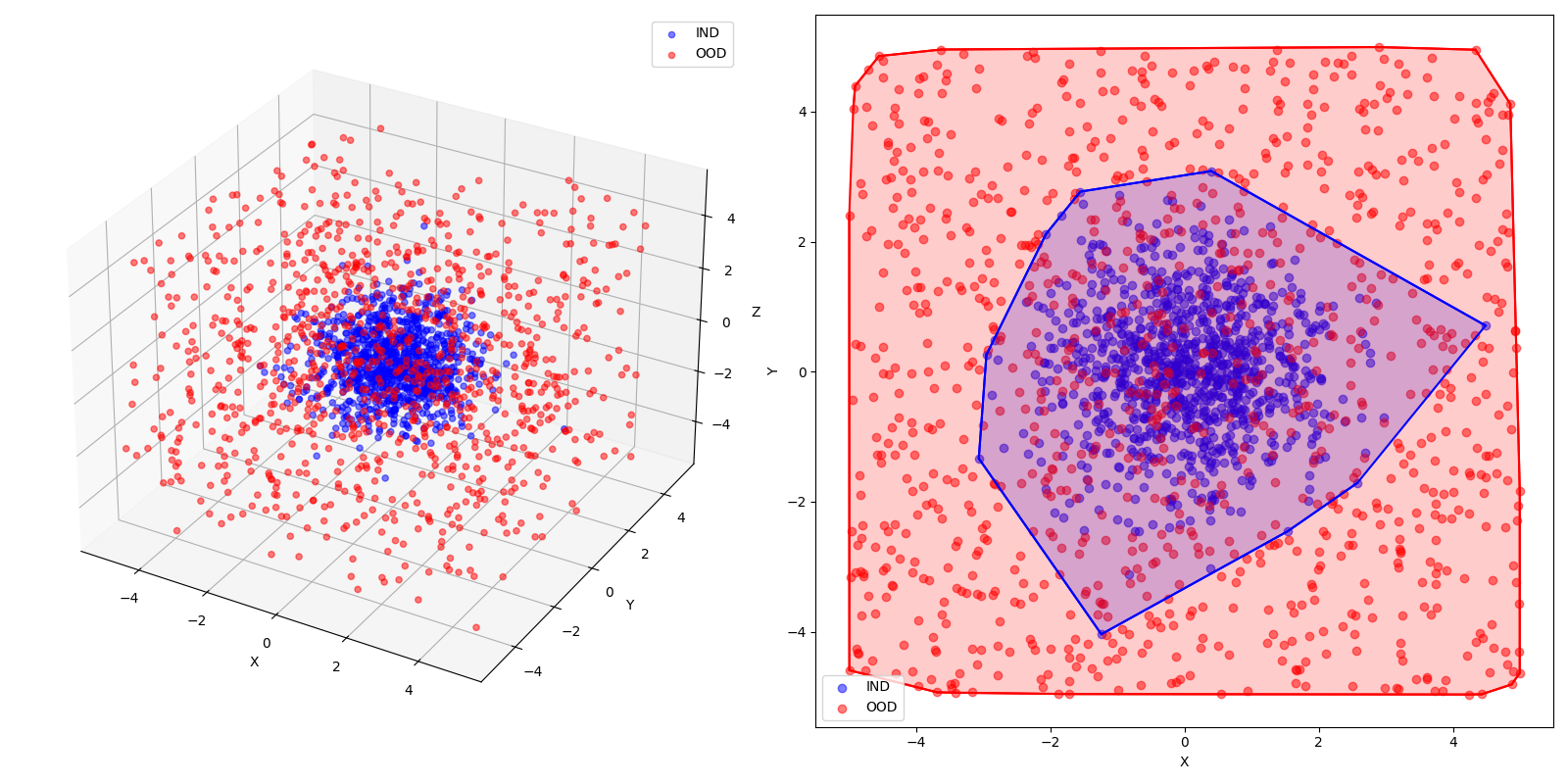
Now, imagine we have Guassian clusters as our IND data and a Uniform distribution as our OOD data. This is how they’d look, assuming a sample size of 1000:

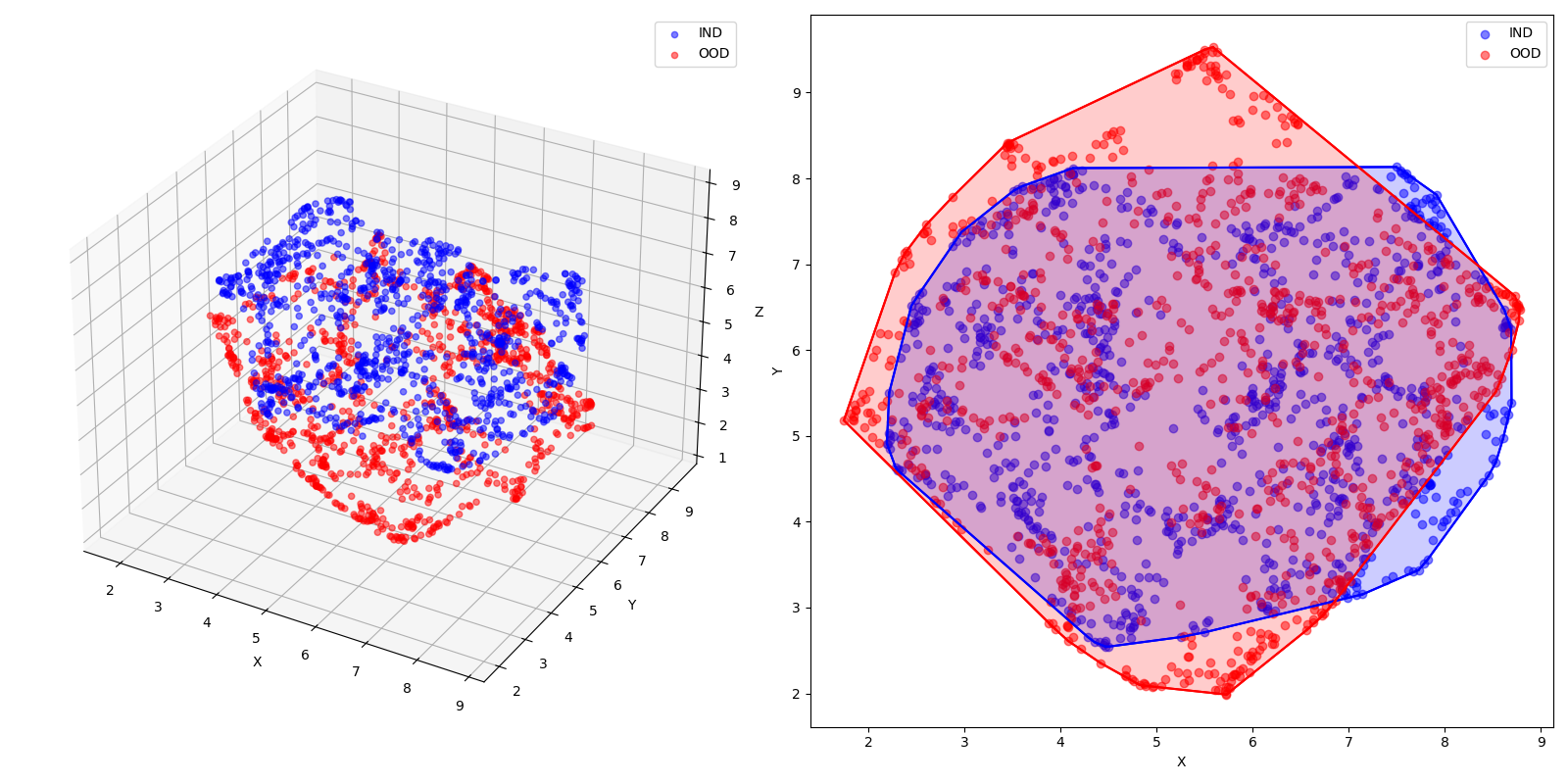
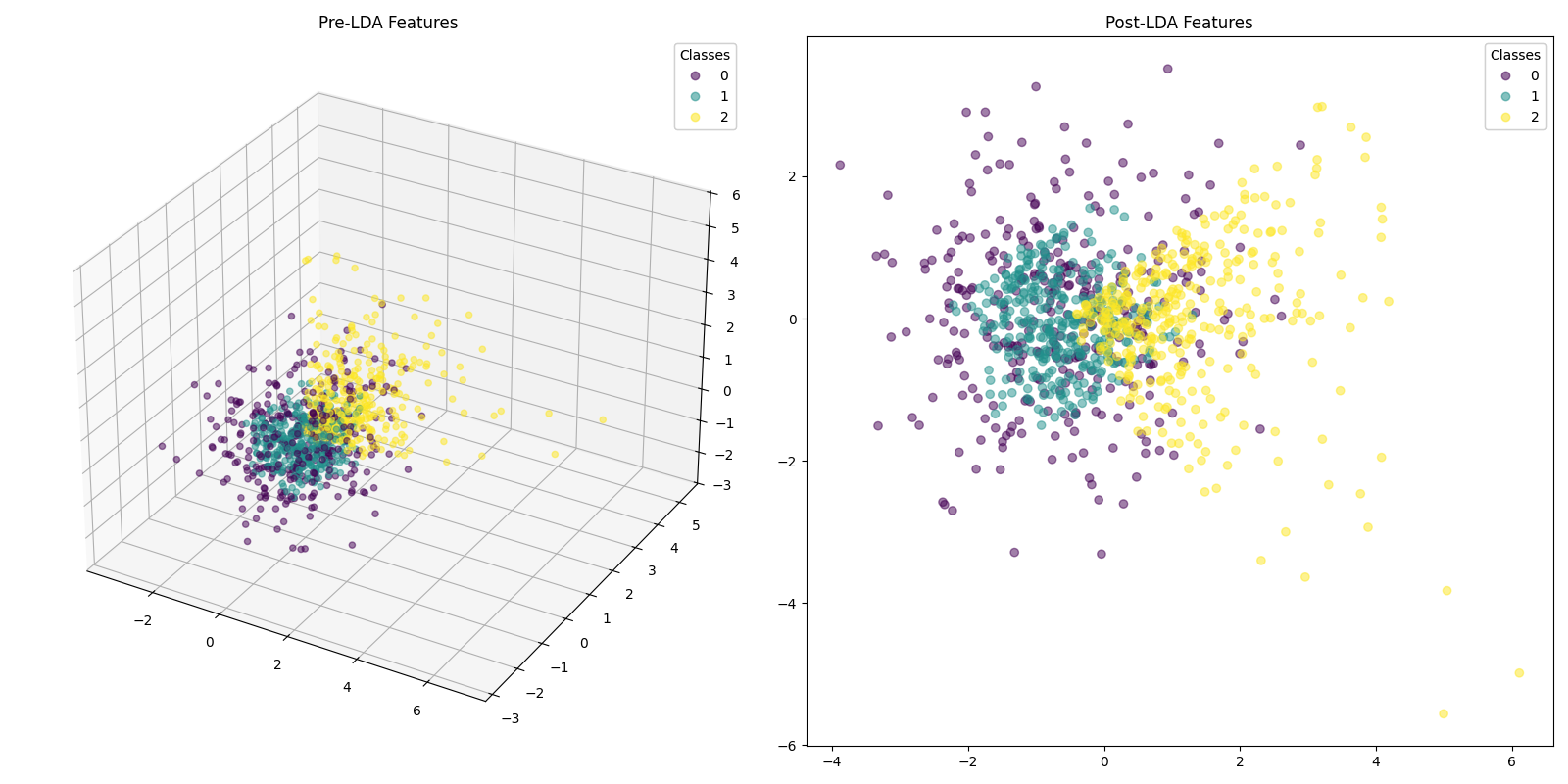
Instead of a whole model, and to ignore the pretext of training, we’ll use PCA for simplicity as an “embedding function”. Here’s how the “extracted” features look:

def extract_features(data, n_components=3):
    pca = PCA(n_components=n_components)
    return pca.fit_transform(data)

We’ll also take the Sum of Squares as the energy function. Here’s how we can find the energy and probability density.

def calculate_energy(features):
    return np.sum(features**2, axis=1)

def calculate_probability_density(energy):
    exp_neg_energy = np.exp(-energy)
    return exp_neg_energy / np.sum(exp_neg_energy)

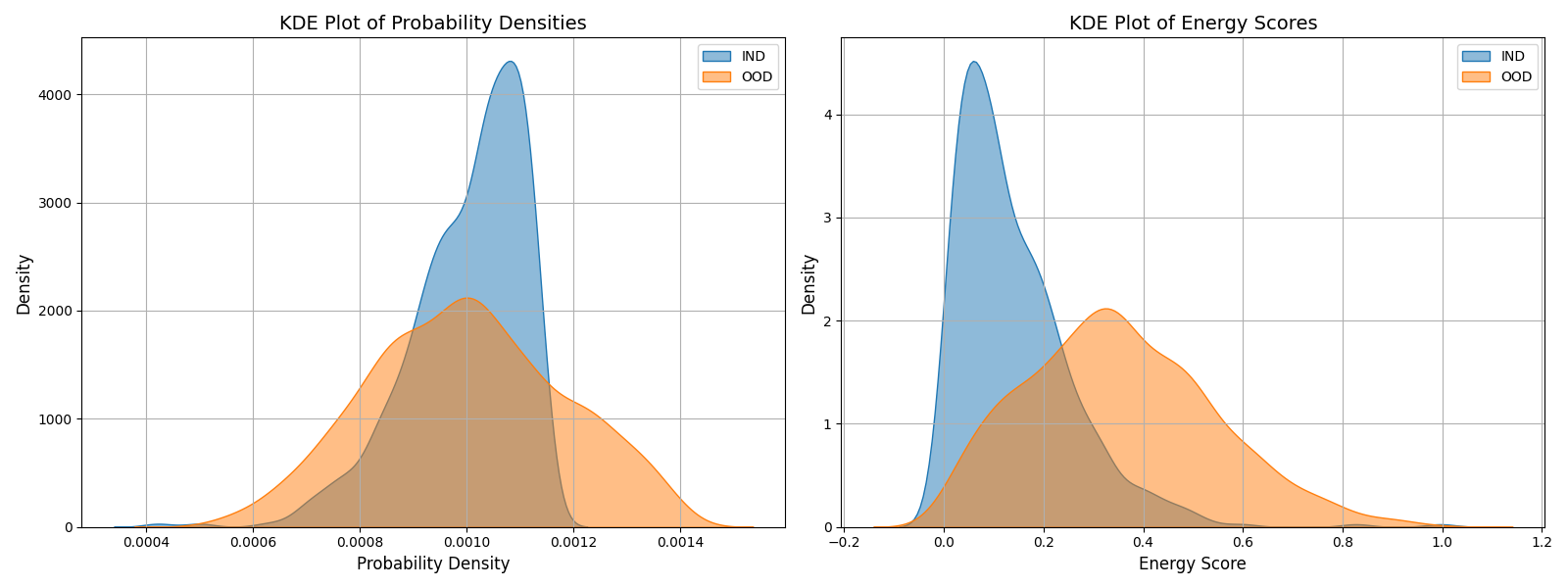
Now, let’s see how these distributions look as a KDE plot:

Note:

• When looking at the energy scores, the KDE plot show that IND samples have lower energy (peak towards the left) while OOD samples have a higher energy (peak towards right). This validates the initial hypothesis.
• When looking at the probability densities, the KDE plot shows that INR samples have higher densities (shifted towards right) while OOD samples have lower density (peak towards left). This confirms the method of using Gibbs.

This method is employed practically for the following examples:

Classification Score (\(S_{cls}\)):

The Classification score projects the extracted features into a discriminative space, and tries to maximize the seperability between the classes. Then, by taking the average of the posterior probabilities of each class being predicted from this projection, it tries to guage how well the features (with minimized inter-class variance) align with the target dataset’s classes.

Note that the energy function here is \(\mathbf{U}^T (\mathbf{f}_i^{(y_i)} - \mu_{y_i})\). The classification score normalizes the discriminant scores (mat-mul of the projected matrix against the normalized feature column) across all classes to compute a posterior probability for the true class.

Here is an optimal view of the method:

where,

• \(\mu_{y_i}\): mean feature vector for the class (y_i).
• \(\mathbf{U}\): projected feature matrix
• \(e^{\mathbf{U}^T (\mathbf{f}_i^{(y_i)} - \mu_{y_i})}\): discriminant score for the true class (y_i).
• \(\frac{e^{\mathbf{U}^T (\mathbf{f}_i^{(y_i)} - \mu_{y_i})}}{\sum_{c=1}^{C} e^{\mathbf{U}^T (\mathbf{f}_i^{(c)} - \mu_c)}}\): normalized posterior probability for the true class (y_i). This fraction represents how well the \(i\)-th sample is classified into its true class compared to other classes.

First, consider a dataset of 1000 samples, with equal sets of Gaussian, Uniform and Exponentially sampled points. Each distribution type is assigned a class. This is how we ideally expect the data modelling to be, so that there is an ability to differentiate the features statistically.

gaussian_embeddings = npr.normal(loc=0.0, scale=1.0, size=(num_samples, dim))
uniform_embeddings = npr.uniform(low=-1.0, high=1.0, size=(num_samples, dim))
exponential_embeddings = npr.exponential(scale=1.0, size=(num_samples, dim))

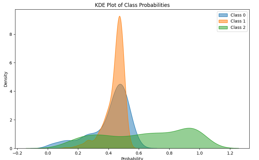
Now, take a look at how the probabilities get distributed when we treat the discriminant scores at the energy function:

Note:

• Class 0: A peak near a probability of 0.5 with a good spread towards lower probabilities. This indicates that the model is less confident in distinguishing Class 2, and there might be more misclassifications.
• Class 1: A sharp peak near a probability of 0.4, with a narrow spread. This indicates that most samples assigned to Class 1 have high probabilities, and the model is confident in these predictions.
• Class 2: A distinct spread with a local peak at 0.9. This would indicate that the model is able to confidently classify in only few of the cases. In the rest of them, it is unable to distinguish the class properly.

From this, we can take a normalized average and use it as a score to estimate the overal confidence of the model. A model with high \(S_{cls}\) would have narrow spread, tall peaks towards the right.

Regression Score (\(S_{r}\)):

The goal of this score is to understand how well the bounding boxes can be reconstructed using the features, assuming a linear relationship by SVD. The regression score is the MSE between the real and predicted \(j\) values for each bounding box \(k\). Lower the score, the better the model will be.

where,

• \(K\): #bounding_boxes
• \(b_k^{(j)}\): \(j\)-th coordinate of the \(k\)-th bounding box’s true label.
• \(\hat{b}_k^{(j)}\): \(j\)-th coordinate of the \(k\)th bounding box’s predicted label,

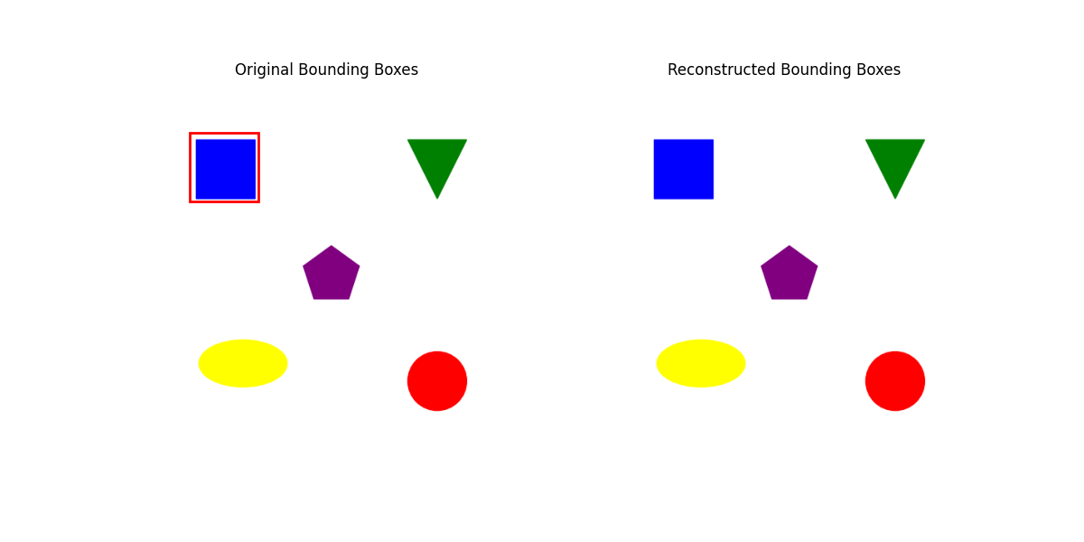
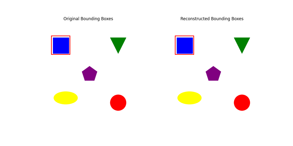
To visualize how this works, we’ll replicate the paper’s methodology, but ignoring the truncation to retrain only 80% of energy values. We will see why I did this in the When (does it fail)? section.

In my naive example, I’m using CLIP’s embedding function from this link to generate features from this image. We’ll focus on a bounding box for the top-left square.

U, S, Vh = torch.linalg.svd(features, full_matrices=False)

energy = torch.cumsum(S**2, dim=0) / torch.sum(S**2)
S_inv = torch.diag(1.0 / S)
features_pseudo_inv = Vh.T @ S_inv @ U.T
bboxes_approximated = features @ features_pseudo_inv @ targets.float()

regression_score = -torch.sum((targets - bboxes_approximated) ** 2) * (1/(targets.shape[0] * 4))[[ 69.99993  64.99993 159.99983 154.99985]]

When (does it fail)?

Dealing purely with \(S_{en}\) is unreliable. This only interfaces between target \(y_{t}\) embeddings and the \(\phi\) embedding functions.

• Consider a PTM trained on a source dataset \(y_{s}\) whose features closely matches the target dataset (imagine two datasets with a lot of cat pictures). Now, if you get the energy score for this (\(\phi, y_{t}\)) pair, the \(E(x, y_{t})\) score will be low, and thus high likelihood.
• However, we’re completely ignoring the rest of the network and the classification labels. Different PTMs with similar embedding layers might be clustered together, regardless of their accuracy.
• Thus, use classification based scores like LogME, LEEP, PACTran and \(S_{cls}\) in addition to the \(S_{en}\) score. Reference the following table to note that \(S_{en}\) does not outperform the combined metrics.

\(S_{cls}\) makes a number of assumptions, which might not hold good in the following cases:

• LDA assumes that the features within each class are normally distributed in the discriminative space: \(\mathbf{\bar{f}}^{(c)} \sim \mathcal{N}(\mathbf{U}^T \mu_c, \mathbf{I})\). The projections might not accurately reflect the seperability in this case.
• When the #dim » #samples_per_class, the variance matrices calculated will ill-conditioned. It will consequently not be positive semidefinite, and thus is unreliable. It will also lead to underflow errors.
• If the feature distributions of different classes significantly overlap, the LDA projection will not clearly separate these classes. This overlap can lead to ambiguous posterior probabilities, as the model will not be confident about class distinctions.

\(S_{r}\) also makes a few assumptions:

• SVD assumes that the relationships between features and labels can be approximated lienarly. This might oversimplify complex non-linear relationships in real-world data.
• If we truncate 80% of singular values, it might lead to a loss of information and thus inability to reconstruct the boxes as needed. For example, consider the same example above, but with 80% truncation. On the right, we see no bounding box plotted. This is because the approximated values are \([0,0,0,0]\). If the remaining singular values don’t adequately represent the features needed to reconstruct the bounding boxes, the reconstruction could default to something uninformative, like the origin.