lightning wildfire lab
Can we predicting wildfires using lightning data? ⚡
- Systematized the process of bundling netCDF data on the basis of temporal, spatial and spatio-temporal features to package into Ensemble, LSTM and ConvLSTM models.
- Responsible for supervising code development and organizing research flow within the lab; Handling evaluation and integration of new scripts to make an efficient system for other researchers to query and visualize information
- Developed scripts using Xarray and Geopandas to package LandSAT data from NASA/NOAA satellites; Used Rasterio to visualize and plot GeoTIFF datasets for analyzing lightning causation
I worked on the Data Handling team as Lead under Michael Wang (NASA) (PI: Yuan Wang (Stanford X NASA)). Our goal was to replicate DeepCube’s Use Case 3, but with a lightning-based focus. Some of my code: GOES-R Scraper + Visualizer, LandSAT Burner Area Finder, Extracting grids from ERA5, USGS Pkg Fork.
Building upon this, I pitched a proposal to the folks at Ambee – in Spring ‘23 – for a related project. You can read more about what I did with Ambee here.
Background
Wildfires are caused by the complex interactions of the fire drivers (weather conditions, land and vegetation characteristics, human activities).
- Weather conditions: Lightning and Thunderstorms, Wind, Heat, High atmospheric temperatures and low humidity, etc.
- Land characteristics: Droughts and dry seasons (soil), vegetation (naturally flammable), etc.
- Human activities: Campfires left unattended, the burning of debris, equipment use and malfunctions, negligently discarded cigarettes, and intentional acts of arson.
According to federal data cited (Wildland Fire Management Information (WFMI)) by the National Park Service, humans cause about 85 percent of all wildfires yearly in the United States. Using data from the National Interagency Fire Center (NIFC), the picture attached below outlines the statistics of human-caused and lightning-caused wildfires.
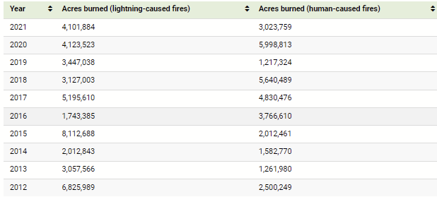
Lightning is the second most common cause of wildfires (behind human causes); thus, predicting the location and timing of future storms and strikes is of great importance to predicting fire occurrence. Here’s a discussion on a fire ignition factors across landscape types.
Drought (and in-turn, land vegetation) has a very complicated relationship with wildfire. Both these factors are not, in and of themselves, the trigger for a wildfire to begin, but it most defintely plays a big role in its persistence.
“Fire depends on two things: having enough fuel and drying that fuel out so it can catch fire. So in the short term, more droughts probably mean more fire as the vegetation dries out,” said Cook. “If those droughts continue for a long period, like a megadrought, however, it can actually mean less fire, because the vegetation will not grow back as vigorously, and you may run out of fuel to burn. It’s definitely complicated.” https://climate.nasa.gov/news/2891/a-drier-future-sets-the-stage-for-more-wildfires/
Previous Research
(Caption: Going over some interesting methodologies used.)
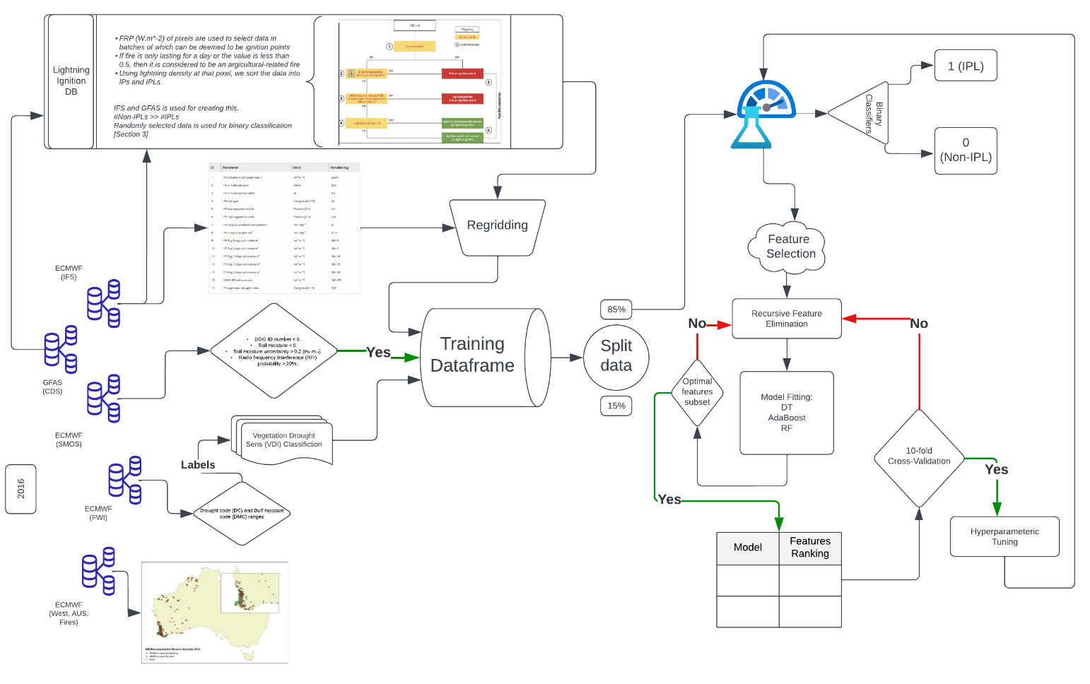
- Using machine learning to predict fire-ignition occurrences from lightning forecasts
- Data:
- Global Fire Assimilation System (GFAS) data has analyzed using Fire Radiative Power (FRP) to find which points in a data field have more temperature over a period of time over it’s surroundings
- Decision Tree is used to iteratively find new IPs
- Those spread to different areas
- Coming in from diff areas
- Fuel ignition is rarely dependent on the fuel moisture of the area and the soil, but the sustainability of it is highly dependent.
- Soil Moisture and Ocean Salinity (SMOS) is used for finding soil moisture and is used as a tuning parameter rather than a variable since “simplicity of the land surface schemes” make it inappropriate to be used towards the same end.
- “Data are available in swath segments on the ISEA 4H9 grid, with grid data provided as discrete global grid (DGG) points, only available along the satellite track with a nominal resolution of 15 km.”
- Low Fuel Moisture situations:
- DC and DMC has duff moister code and corresponding moisture data of deep, organic layers until 10cm depth.
- Data is classifid based on ranges
- Identified parameters with EDA plots:
- 2m temp
- 2m relative humidity
- vegetation coverage
- soil type
- Method:
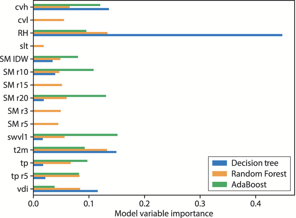
- Decision Trees with Adaboost vs RF
- DT and RF both give 2m RH and t2m
- Low ranking params like those above (in the data section) are not considered
- Analyzing how to find model’s optimal performance estimates:
- Assumes the cloud to ground density product is accurate
- Assumes all non-IPLs are removed
- An RFE (recursive feature elim) is used to recursively cut down on the 15 features that are considered for training
- Consider’s smaller and smaller set of variables where it estimates the importance of each variable
- Procedurally removes features which aren’t used to make key decisions
- CV (cross validator) is used instead of simple test train split
- Splits into train and validation
- k iterations of training
- Within each, one fold is held out to train on all other validation sets
- Hyper-parameterization using scikit-learn
- GridSearchCV was used for the boosting algoritms (Adaboost)
- RandomSearchCV was used for bagging (RF)
- Decision Trees with Adaboost vs RF
- Data:
- Near Real-Time Wildfire Progression Monitoring with Sentinel-1 SAR Time Series and Deep Learning
- Data:
- SARs (Synthetic Aperture Radar) data used for the following fires:
- the 2017 Elephant Hill Fire in British Columbia, Canada,
- the 2018 Camp Fire in California, USA, and
- the 2019 Chuckegg Creek Fire in northern Alberta, Canada.
- SARs (Synthetic Aperture Radar) data used for the following fires:
- Method:
- Pre-processing the raw SAR files before and after fire has begun in order to detect area changed by the wildfires
- Binary mask using time series anomaly detection
- Data split and used to train the CNN to be fitted to the burned area map and generate a burn probability mask
- The outputs of the CNN refinement are CNN burnConf maps, where the pixel values are ranging from 0 to 1 and they are proportional to the probability that each pixel represent a burnt area (0: unburnt, 1: burnt).
- Such data is already provided by Landsats BA L3 product.
- Otsu’s thresholding is used to threshold the points from the background
- Notes:
- SAR is used cuz it allows for cloud penetration and doesn’t depend on the solar radiation like landsat does.
- VIIRS and MODIS has a lower res than GOES, but more spectral band and a higher frequency of rev
- Data:
Initial Analysis
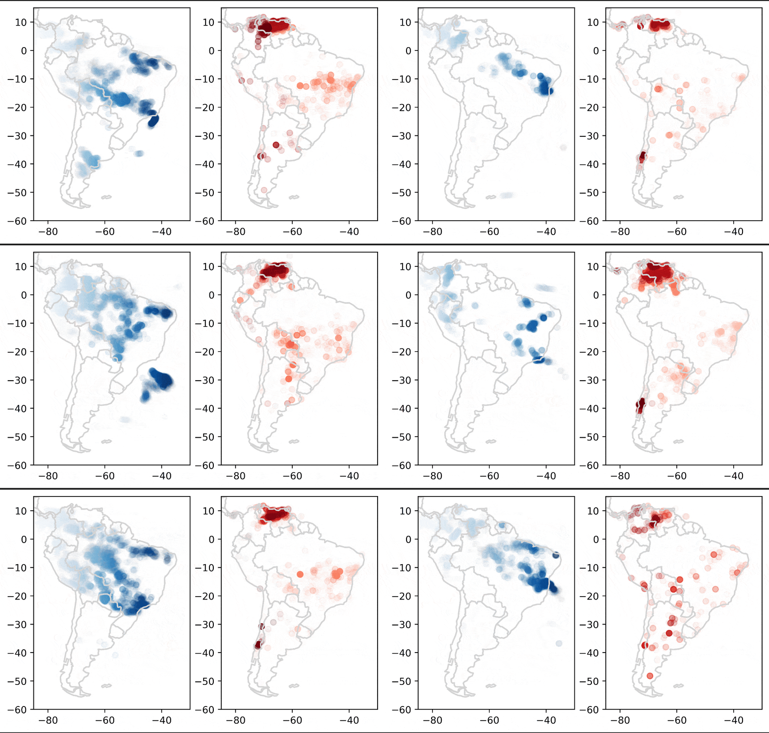
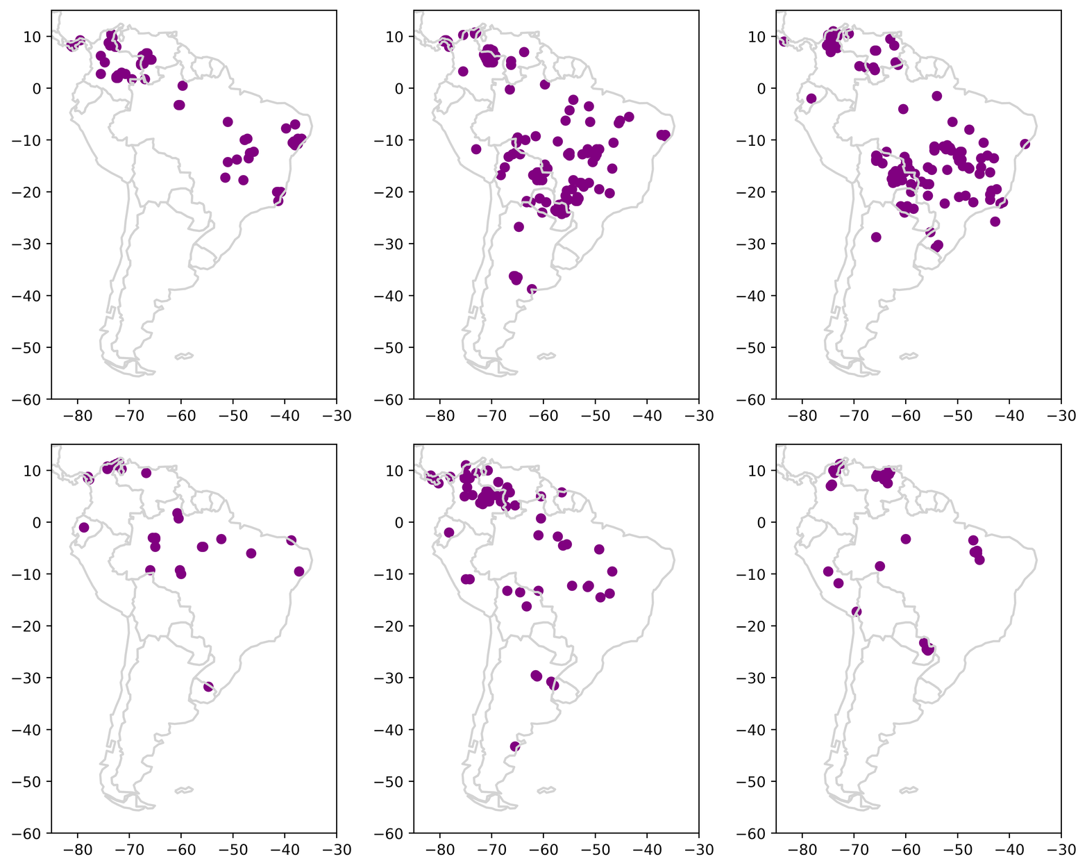
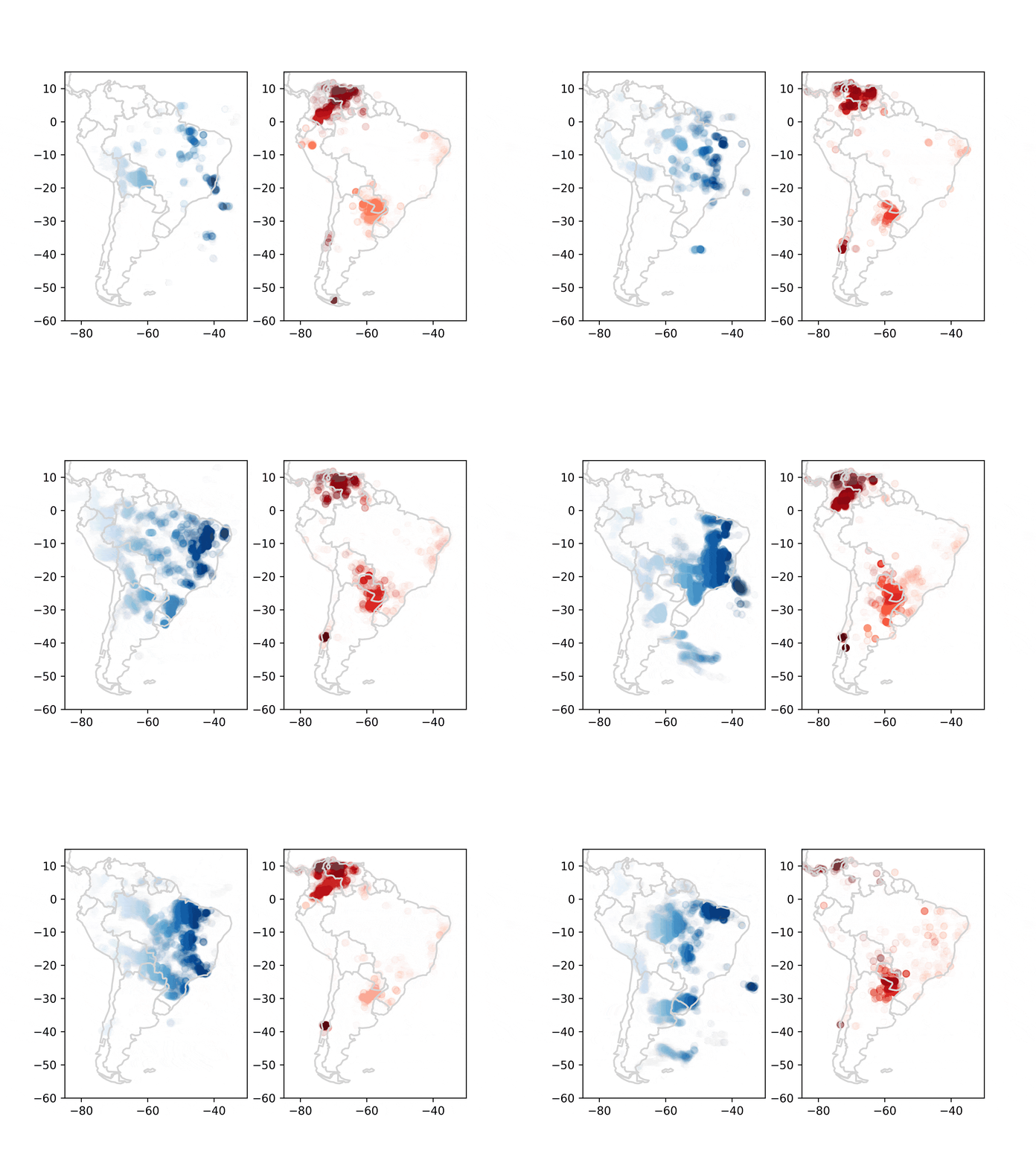
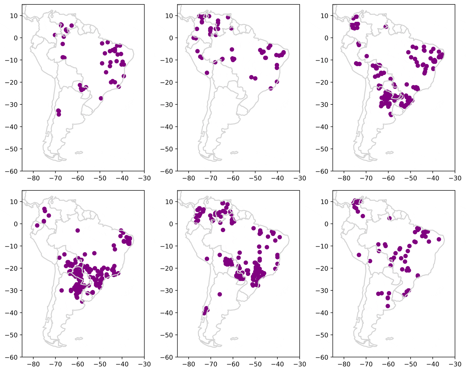
To have a more concrete understanding of the relationship between lightning and fire, I have conducted a case-study of South America across 2022’s seasons. Here’s a quick brief:
- Collected data for the 4 major seasons in South America (April, Feb, July, Oct) from 2022 (reported record wildfires)
- GOES-R GLM → Lightning Strikes, Historic and NRT
- VIIRS → FRP, Historic and NRT
- ERA5 → Reanalysis weather variables in hourly format, Historic and NRT
- Gridded lightning and fire density products for South America coordinates
- Implemented Lightining-Ignition Classifier
- Classifies coordinates where a fire is known to have taken place, white is not a countinuing fire nor is coming from surrounding areas, and is known to have a storm overhead in a 12-hr lag period
According to this report by Copernicus, Feb has seen record wildfire activities and this report discusses how Catatumbo lightning intensifies over the April - August Period. These two months will be focused on, as they form the main ‘fire’ seasons in South America.
You can find the code for the visualizations and data here.
February 2022
April 2022
Prototype Classifier
Below is the algorithm I used for identifying ‘lightning-ignited fires’ based on GLM and VIIRS (/MODIS) data. It was modelled from the method shown here.
\[\text{Let } G_{ij}^{t} \text{ represent the state of a cell in an } n \times m \text{ canvas grid at time } t, \text{ where } i \text{ and } j \text{ are the row and column indices, respectively.}\] \[G_{ij}^{t} \in \{0, 1\} \text{, where 1 indicates the presence of fire.}\] \[\text{An ignition point at time } t \text{ is defined by: } G_{ij}^{t} = 1 \text{ and } G_{ij}^{t-1} = 0.\] \[\text{Let } L_{ij} \text{ represent the state of a cell in an alternate } n \times m \text{ grid for lightning, with } L_{ij} \in \{0, 1\} \text{ where 1 indicates the presence of lightning.}\] \[\text{An "IPL" (intersection point between fire and lightning) is defined by: } G_{ij} = L_{ij} = 1.\]

Next Steps
Using this data as a base, I’m working on using the IPL point-map as a way to narrow the search for relevant incidents for modelling. I intend to collect and identify correlations between weather-data with the convex-hull region around IPLs to train a binary classifier in a method similar to what is proposed in this paper.
Here’s some data I have acquired and transformed for the purpose. It is modelled after the IFS used by the paper
| IFS (Paper) | ERA5 (Proposed Alt) |
|---|---|
| Volumetric Soil Water Layer | Volumetric soil water layer 1 |
| 2m temp | 2m temperature |
| 2m relative humidity | 2m dewpoint temp [1] |
| soil type | soil type |
| low vegetation cover | low vegetation cover |
| high vegetation cover | high vegetation cover |
| daily accumulated precipitation | total precipitation |
| avg 5 days precipitation | [2] |
| avg 3 days soil moisture | [2] |
| avg 5 days soil moisture | [2] |
| avg 10 days soil moisture | [2] |
| avg 15 days soil moisture | [2] |
| avg 20 days soil moisture | [2] |
| CAPE | Convective available potential energy |
- [1] 2m RH found from Dewpoint Temp*
- [2] calculated post-download*
After that, I want to prose the problem as a forecasting problem with a supervised-learning approach of \(([t-1]^{n*m}, [t]^{n*m})\) predictions. The data needs to be translated into the following structure for it to work with XGBoost:
- Construct a 3-dimensional array (n_samples, time_steps, features) incorporating mean, slope, and variance across a periodicity of 3-4 days to enrich the dataset.
- Transform the dataset into a 2D format (n_samples * time_steps, features), focusing on calculating mean, variance, and slope temperatures for every 3-day segment within a week.
- Reintegrate these calculations into the dataset and revert it to its original 3D structure (n_samples, time_steps, features).
- Finalize the dataset format as [coordinates, n_timesteps * n_features], optimizing it for the intended modeling processes.